elibaum.com

computing pi from flipping coins

05 Apr 2025

Say you need a handful of binary strings to have distinct Hamming weights (hypothetically). What is the probability this occurs for random strings of a certain length? The answer is extremely surprising: it gives an extremely imprecise method for computing \(\pi\)!

Let’s just consider the case of two random binary strings \(s_0,s_1\) of length \(n\). The probability that \(\mathsf{wt}(s_0)=\mathsf{wt}(s_1)\) is equal to the sum of the probabilities that \(\mathsf{wt}(s_0)=\mathsf{wt}(s_1)=t\), for all \(t\in[0,n]\). Each of these terms is a simple binomial expression:

\[\Pr[\mathsf{wt}(s_0)=\mathsf{wt}(s_1)]=\sum_{t=0}^n\Pr[\mathsf{wt}(s_0)=\mathsf{wt}(s_1)=t]=\sum_{t=0}^n \left(\frac{\binom n t}{2^n}\right)^2\]

By a nice binomial identity, \(\sum_{t=0}^n\binom n t ^2 = \binom{2n} n\) To see this, imagine we put \(s_0, s_1\) side by side, and flip all of the bits in the second half. Now we ask: what is the probability that this \(2n\)-bit string has \(t\) ones in the first half, and \(t\) zeros in the right half? Then there are \(n-t\) ones in the second half, or \(n\) ones overall out of \(2n\) total bits.

At this point, we can also imagine the setup as asking for the probability of a tie between heads and tails after flipping a coin an even number of times (\(2n\)).

Simplifying a bit:

\[\Pr[\text{same HW}]=\frac{\binom{2n} n}{2^{2n}}=\frac{(2n)!}{(n!2^n)^2}\]

which looks relatively innocuous.

Taking Stirling’s approximation, \(n!\approx \sqrt{2\pi n}\left(\frac n e\right)^n\), we can argue that for large \(n\), this probability is, improbably,

\[\begin{align} \Pr[\text{same HW}]=\frac{(2n)!}{(n!2^n)^2}&\approx\frac{\sqrt{4\pi n} (2n/e)^{2n}}{2\pi n (n/e)^{2n}\cdot 2^{2n}}\\ &=\frac{2^{2n}n^{2n}e^{2n}}{\sqrt{\pi n}n^{2n}e^{2n}\cdot2^{2n}}\\ &=\frac{1}{\sqrt{\pi n}} \end{align}\]

Where does \(\pi\) come from here? Stirling’s approximation, sure, but in the scenario there’s nothing that even looks remotely close to a circle.¹

We can also show the above equivalence via Wallis’s integral, which defines

\[W_n := \int_0^{\pi/2}\sin^n x\,dx\]

Various identities are known, including, for even arguments:

\[\begin{gather} W_{2n} = \frac{\Gamma(n+1/2)\Gamma(1/2)}{2\Gamma(n+1)}\\ W_{2n} = \frac{(2n)!}{(n!2^n)^2}\cdot \frac \pi 2 \end{gather}\]

The latter identity looks close to what we have. Rearranging gives

\[\Pr[\cdot] = \frac{(n-1/2)!}{n!\sqrt{\pi}}\]

Note that this is an exact result, relying on the gamma function to extend factorials to the reals. We can next use Stirling’s again to argue

\[\frac{(n+a)!}{n!}\sim n^a\]

and thus \(p\approx 1/\sqrt{\pi n}\).

But this is not very satisfying.

Looking for the circle

The most immediate place place to start looking is by rearranging into an area formula: \(p = 1/\sqrt{\pi n}\) so \(1/n = \pi p^2\). The interpretation: I flip a coin \(2n\) times. What is the probability of a tie? Draw a circle with area \(1/n\). Its radius \(p\) will give the approximate probability…

We can think of this smaller circle (area \(1/n\)) lying inside a larger circle of radius \(1\) (and thus, in the radius-as-probability model, it contains all possible outcomes). The large circle has area \(\pi\), and the smaller circle contains a \(\frac 1 {\pi n}\) fraction of the total area. Maybe, in some sense, by sampling random binary strings (or flipping coins) we are picking uniform points along an arbitrary radius. That doesn’t really make sense though. Or, imagine tracing out a curve in polar coordinates, with \(\theta=2\pi x/2^n\) and \(r~\mathsf{wt}(x)\), and then taking an average? However, it’s not clear that polar coordinates actually get us anything here; this seems equivalent to just taking the average value of the Hamming weight over all \(n\)-bit strings.

3b1b has an excellent video on a geometric interpretation of the Wallis product for \(\pi\), which, while closely related to the Wallis integral, is not clearly connected to this setting, at least as far as I can tell. But the circle there was pretty well hidden.

Another not-quite-fleshed out idea: consider a circle, now with area \(1\) (and radius \(1/\sqrt\pi\)). Draw a smaller circle with area \(1/2\) (radius \(1/\sqrt{2\pi}\)). Random points inside the small circle are “more heads than tails” outcomes and points outside the small circle are “more tails than heads”. Now we draw a thin strip along the boundary circle, with area \(1/\sqrt{\pi n}\): this is the probability of a tie. I thought a bit about tiling the larger circle with a bunch of tin (sorted) coins, and then asking where the first H T occurs. But imposing ordering on the coins asks a very different question, and I really don’t see a satisfying connection here.

If you have another idea, please email me: i.found.the.pi@elibaum.com

The normal distribution

View the random bits, or coin flips, as uniformly random samples drawn from \(\{1,-1\}\). Then we are interested in the probability that \(2n\) such values sum to 0.² With large \(n\), the Central Limit Theorem tells us that this should converge to the normal distribution — and in that framing, the value we are interested in is the PDF of the normal distribution at \(x=0\). The PDF is

\[f(x) = \frac 1 {\sqrt{2\pi\sigma^2}} \exp\left(-\frac{(x-\mu)^2}{2\sigma^2}\right)\]

\(\mu=0\), by symmetry, and the variance can be approximated from the binomial distribution: \(\sigma^2=np(1-p)\). Here, our domain is actually \(2n\), so \(\sigma^2=2n(1/2)^2=n/2\). Then

\[f(0)=\frac 1{\sqrt{\pi n}}e^0=\frac 1{\sqrt{\pi n}}\]

I’m not sure if that’s any more convincing, but it’s something.³ This way of looking at the problem also gives a more general way of approximating \(\pi\), given any final sum, not just zero.

Computing \(\pi\)

Above, we found \(p \approx 1/\sqrt{\pi n}\), so \(\pi \approx 1 / np^2\) for a coin flipped \(2n\) times. If we run \(T\) trials, and \(c\) of them have a tie,

\[\pi \approx \frac{T^2}{nc^2}\]

This is a pretty bad approximation. Here’s a snippet to run the estimator:

flips = np.random.randint(0, 2, size=(2*n, TRIALS))
ties = np.cumsum(sum(flips) == n)

est = (np.arange(TRIALS) / ties) ** 2 / n

I tested this with n = 100:

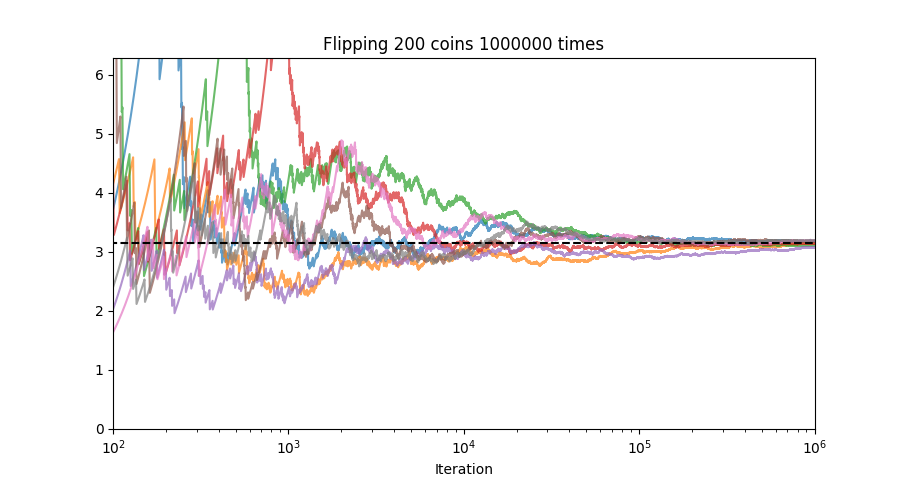
Even after one million iterations, we’re just barely getting close to \(\pi\):

Granted, you could get better convergence by considering all outcomes (instead of just ties), drawing the curve, and trying to fit a normal distribution. Part of the slow convergence is that the odds of getting a tie in the above scenario are only around 5%, so the vast majority of iterations don’t contribute anything to the estimate. Furthermore, while the approximation only holds for large \(n\), the probability of a tie gets smaller and smaller, so convergence slows…

Of note: Eric Postpichil asked a similar question almost 30 years ago, and gave a similar analysis.

---

1. This question is loosely inspired by 3b1b’s colliding-block video, where he shows how a mysterious computation of \(\pi\) does, actually, connect to a circle hidden in the physics. ↩

2. Or view this setup as a Galton Board, where we are interested in the relative height of the central column. ↩

3. Of course, 3b1b also has a video on where this \(\pi\) in the normal distribution comes from. It’s a nice geometric construction in 3D, but I can’t quite relate it to the coin flipping problem yet. I think the lesson here is that 3b1b has already published videos answering the questions I haven’t yet asked. ↩